日志

磁场强度和拉莫尔半径

粒子的拉莫尔半径为

$$R=\frac{\gamma mv}{qB}= 1.7\times10^{7}\gamma(\frac{v}{1c})(\frac{B}{1\mu G})^{-1}m\approx 10^{10}m\ll 1pc=3\times 10^{16}m$$

远小于云团的尺寸。其中磁场满足：

$$\bar{B}=3.8\mu G$$

假定（Ching et al 2022）

$${B}=(3.8+0.3\times rand())\mu G$$

那么粒子的偏转半径为：

$$\Delta \theta=\frac{c\Delta t}{R}=\frac{3\times 10^8 \times \Delta t}{1.7\times10^{7}\gamma}*(3.8+0.3\times rand())*rand()$$

其中$\gamma=1000$。为了保持误差在一定范围内：

$$\Delta \theta \leq1 \Rightarrow \Delta t\leq100s$$

这对于以Myr为单位的计算是困难的，因为：

$$1Myr=3\times10^{13}s$$

意味着要进行$3\times10^{11}$次计算，想想就可怕。

为了解决这个问题，只能避开模拟的方法，通过扩散模型将其时间尺度拉到与云团尺度匹配的数量级。

云团尺寸

对云团的尺寸没有定论，假定

$$\bar{L}=1pc$$

扩散模型

一束粒子在原点散开，其分布满足怎么样的模型？由于相当于加速度空间的随机游走，且最终时间尺度很大，我推测其接近简单的扩散模型，需要测定扩散的系数。

扩散模型指出：

$$P(x,y,z,t)=\dfrac{1}{(4\pi D t)^{\frac32}}\exp{[-\dfrac{x^2+y^2+z^2}{4Dt}]}=\dfrac{r^2 }{2\sqrt{\pi}(Dt)^{\frac32}}\exp{[-\dfrac{r^2}{4Dt}]}$$

我们通过模拟来测定该系数$D$。为了保证消除初始方向的影响，总时间不能太少；为了消除涨落的影响，总数不能太少。

粒子的运动函数为：

function [particle_velocity,particle_position]=movement_func(N,particle_position,particle_velocity)
theta=3/1.7*(3.8+0.3*rand(1,N)).*rand(1,N)*timestep*10./particle_gamma;
particle_velocity_new=rotation(particle_velocity,theta);
particle_position=particle_position+timestep*(particle_velocity+particle_velocity_new)/2;
particle_velocity=particle_velocity_new;
end

在磁场中的旋转函数为：

function v_rotated = rotation(v, theta)
    % v is a 3xN matrix where each column is a vector to be rotated
    % theta is a 1xN vector where each element is the rotation angle for the corresponding vector in v

    % Initialize the rotated vectors matrix
    v_rotated = zeros(size(v));
    
    % Loop over each vector and its corresponding angle
    for i = 1:length(theta)
        random_vector = rand(3,1) - 0.5;
        axis = random_vector / norm(random_vector);

        K = [0, -axis(3), axis(2); axis(3), 0, -axis(1); -axis(2), axis(1), 0];
        I = eye(3);
        cos_theta = cos(theta(i));
        sin_theta = sin(theta(i));
        rotation_matrix = cos_theta * I + (1 - cos_theta) * (axis * axis') + sin_theta * K;

        % Rotate the current vector and store it in the rotated vectors matrix
        v_rotated(:, i) = rotation_matrix * v(:, i);
    end
end

总的代码为：

clc
close all
clear all

%% Generate delta probability
N=10000;
timestep=10;
particle_position=zeros(3,N);
particle_velocity=zeros(3,N);
particle_velocity(1,:)=1;
particle_gamma=zeros(1,N);
particle_gamma(1,:)=1000;

%% Simulation
total_time=1e5;
time=round(total_time/timestep);
for i=1:time
    [particle_velocity,particle_position]=movement_func(N,particle_position,particle_velocity);
end

figure()
scatter3(particle_position(1,:),particle_position(2,:),particle_position(3,:))

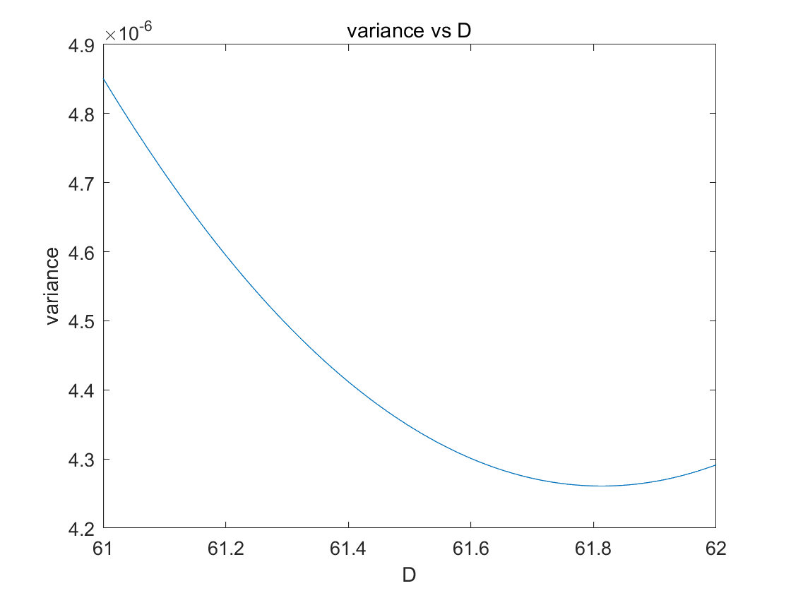
测定代码为：

close all
points=particle_position;
distances_squared = sqrt(sum(points.^2, 1));
num_bins = 20;
[counts, edges] = histcounts(distances_squared, num_bins, 'Normalization', 'probability');
mid_points=(edges(2:end)+edges(1:end-1))/2;


variance=zeros(10,1);
D=linspace(61,62,100);
for i=1:100
    Dt=D(i)*1e5;
    variance(i)=var(counts-gauss(edges,Dt));
end
figure()
plot(D,variance)
xlabel('D')
ylabel('variance')
title('variance vs D')

result=gauss(edges,6.18e6);
figure()
plot(mid_points,counts)
hold on
plot(mid_points,result)
xlabel('r')
ylabel('p')
title('probability vs r')


function result=gauss(edges,D)
result=zeros(1,size(edges,2)-1);
func=@(x) (exp(-x.^2./4./D).*x.^2./2./sqrt(pi)./D.^1.5);
for i=1:size(edges,2)-1
result(1,i)=integral(func,edges(i),edges(i+1));
end
end

结果为：

$$D=61.8$$

图示：

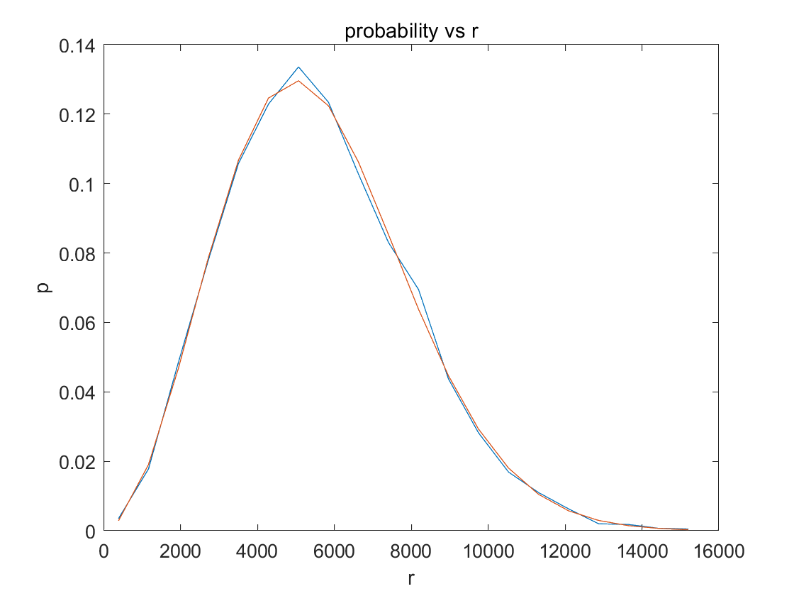
同时也证明了其分布符合扩散模型。

扩散系数和磁场强度的关系

通过以下代码进行试探：

clc
close all
clear all

D_save=zeros(10,1);
B_list=linspace(3,5,10);
for i=1:10
    B=B_list(i);
    N=10000;
    timestep=10;
    particle_position=zeros(3,N);
    particle_velocity=zeros(3,N);
    particle_velocity(1,:)=1;
    particle_gamma=zeros(1,N);
    particle_gamma(1,:)=1000;


    total_time=1e4;
    time=round(total_time/timestep);
    for j=1:time
        [particle_velocity,particle_position]=movement_func(B,N,particle_position,particle_velocity,particle_gamma,timestep);
    end


    distances_squared = sqrt(sum(particle_position.^2, 1));
    num_bins = 20;
    [counts, edges] = histcounts(distances_squared, num_bins, 'Normalization', 'probability');
    mid_points=(edges(2:end)+edges(1:end-1))/2;
    D_min = 1;
    D_max = 200;
    tol = 1e-3;

    optimal_D = find_optimal_D(edges, counts,total_time, D_min, D_max, tol);

    D_save(i,1)=optimal_D;
end

figure()
plot(B_list,D_save)

function optimal_D = find_optimal_D(edges, counts, t, D_min, D_max, tol)
    % 定义方差函数
    variance_func = @(D) variance_counts(D, t, edges, counts);
    
    % 均匀采样D值
    num_samples = 1000; % 可以根据需要调整采样数量
    D_samples = linspace(D_min, D_max, num_samples);
    variances = arrayfun(variance_func, D_samples);
    
    % 找到最小方差对应的D值
    [min_variance, idx] = min(variances);
    initial_optimal_D = D_samples(idx);
    
    % 确定二分法的搜索范围，围绕最小方差点的一个小区间
    D_search_range = [max(D_min, initial_optimal_D - 10), min(D_max, initial_optimal_D + 10)];
    
    % 使用二分法在最小方差附近寻找更精确的D值
    optimal_D = [];
    current_min_variance = min_variance+1;
    D_min_search = D_search_range(1);
    D_max_search = D_search_range(2);
    
    while (D_max_search - D_min_search) > tol
        D_mid = (D_min_search + D_max_search) / 2;
        current_variance = variance_func(D_mid);
        
        if current_variance < current_min_variance
            current_min_variance = current_variance;
            optimal_D = D_mid;
        end
        
        if current_variance < variance_func(D_max_search)
            D_max_search = D_mid;
        else
            D_min_search = D_mid;
        end
    end
    
    fprintf('Optimal D value: %f\n', optimal_D);
end

function var_counts = variance_counts(D,t, edges, counts)
Dt = D * t;
gauss_counts = gauss(edges, Dt);
var_counts = var(counts - gauss_counts);
end

function result=gauss(edges,D)
result=zeros(1,size(edges,2)-1);
func=@(x) (exp(-x.^2./4./D).*x.^2./2./sqrt(pi)./D.^1.5);
for i=1:size(edges,2)-1
    result(1,i)=integral(func,edges(i),edges(i+1));
end
end

function [particle_velocity,particle_position]=movement_func(B,N,particle_position,particle_velocity,particle_gamma,timestep)
theta=3/1.7*(B).*rand(1,N)*timestep*10./particle_gamma;
particle_velocity_new=rotation(particle_velocity,theta);
particle_position=particle_position+timestep*(particle_velocity+particle_velocity_new)/2;
particle_velocity=particle_velocity_new;
end



function v_rotated = rotation(v, theta)
% v is a 3xN matrix where each column is a vector to be rotated
% theta is a 1xN vector where each element is the rotation angle for the corresponding vector in v

% Initialize the rotated vectors matrix
v_rotated = zeros(size(v));

% Loop over each vector and its corresponding angle
for i = 1:length(theta)
    random_vector = rand(3,1) - 0.5;
    axis = random_vector / norm(random_vector);

    K = [0, -axis(3), axis(2); axis(3), 0, -axis(1); -axis(2), axis(1), 0];
    I = eye(3);
    cos_theta = cos(theta(i));
    sin_theta = sin(theta(i));
    rotation_matrix = cos_theta * I + (1 - cos_theta) * (axis * axis') + sin_theta * K;

    % Rotate the current vector and store it in the rotated vectors matrix
    v_rotated(:, i) = rotation_matrix * v(:, i);
end
end

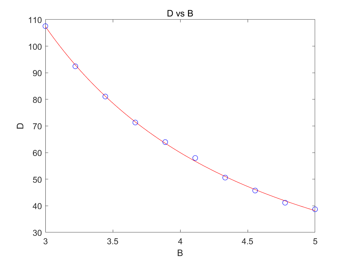
拟合得到

$$D=1000\times B^{-2}$$

扩散系数可以由运动表达式进行推导：

$$D\propto a^2$$

其中a是步长，在磁场内，粒子的步长（平均自由程）为：

$$a\propto R=\frac{\gamma mv}{qB}$$

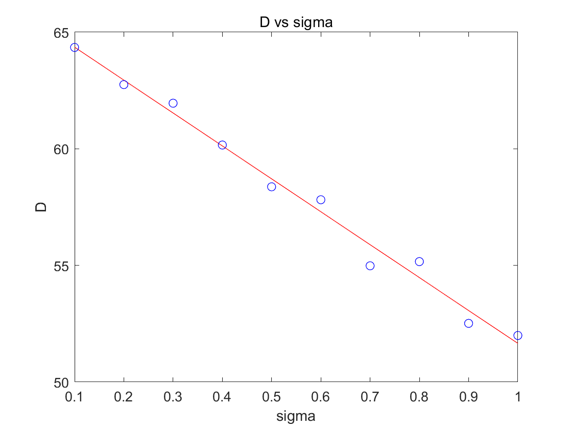
扩散系数和磁场不均匀性的粗略关系

$$B=3.8\pm \sigma \mu G$$

拟合得到

$$D=65.77-14.11\sigma$$

这是符合直觉的，因为不均匀性变相减小了自由程。

费米场的保守性？不均匀性的抵消？

$$\epsilon=\frac{\beta(\cos{\theta_2}-\cos{\theta_1})(1+\beta \cos{\theta_2})}{1-\beta^2}\approx \beta(\cos{\theta_2}-\cos{\theta_1})(1+\beta \cos{\theta_2})$$

该表达式的$(\cos{\theta_2}-\cos{\theta_1})$项决定了其在费米场中闭环积分为守恒的，即势场为一阶保守场；同时一阶不均匀性也相互抵消。

后者指出小范围闭环积分上可视为均匀速度场；前者指出均匀速度场中是保守的。

然而$(1+\beta \cos{\theta_2})$项的后项导致了二阶的不确定性。由于我们的加速是通过二阶加速的，这个不确定性不可忽略。

推导：

能量增加率为

$$\epsilon=\frac{\beta(\cos{\theta_2}-\cos{\theta_1})(1+\beta \cos{\theta_2})}{1-\beta^2}\approx \beta(\cos{\theta_2}-\cos{\theta_1})(1+\beta \cos{\theta_2})$$

在小范围小变角的情况下：

$$\epsilon(\beta,\theta,d\theta)=\beta\sin{\theta}(1+\beta\cos{\theta})d\theta=\beta\sin{\theta}d\theta+\beta^2\sin{\theta}\cos{\theta}d\theta$$

对一个小路线进行积分，有：

$$\begin{aligned} 1+\epsilon &=\prod_{i=1}^{n}(1+\epsilon_i)\\ &\approx\prod_{i=1}^{n}(1-\beta_i \sin{\theta_{i}}d\theta_i-\beta_i^2\sin{\theta_i}\cos{\theta_i}d\theta_i)\\ &\approx1-\sum_{i=1}^n(\beta_i \sin{\theta_{i}}d\theta_i+\beta_i^2\sin{\theta_i}\cos{\theta_i}d\theta_i)\\ &\approx1-\int_{\theta_1}^{\theta_2}\beta_i \sin{\theta_{i}}d\theta_i+\beta_i^2\sin{\theta_i}\cos{\theta_i}d\theta_i\\ &=1+\bar\beta(\cos{\theta_2}-\cos{\theta_1})+\frac14\bar\beta^2(\cos{2\theta_2-\cos{2\theta_1}})\\ &-\int_{\theta_1}^{\theta_2}\delta(\beta)_i \sin{\theta_{i}}d\theta_i-\int_{\theta_1}^{\theta_2}\delta(\beta)_i^2\sin{\theta_i}\cos{\theta_i}d\theta_i\\ &-\int_{\theta_1}^{\theta_2}\beta_i \delta(\sin{\theta_{i}})d\theta_i-\int_{\theta_1}^{\theta_2}\beta_i^2\delta(\sin{\theta_i}\cos{\theta_i})d\theta_i \end{aligned}$$

好消息是在均匀速度场中忽略内部变化情况，得到的能量增加率为：

$$\bar\beta(\cos{\theta_2}-\cos{\theta_1})(1+\bar\beta \cos{\theta_2})$$

比计算内部情况的误差只有

$$\begin{aligned} err_1&=\frac14\bar\beta^2(\cos{2\theta_2-\cos{2\theta_1}})-\bar\beta^2(\cos{\theta_2}-\cos{\theta_1})\cos{\theta_2}\\ &=\frac12\bar\beta^2(\cos^2{\theta_2-\cos^2{\theta_1}})-\bar\beta^2(\cos{\theta_2}-\cos{\theta_1})\cos{\theta_2}\\ &=-\frac12\beta^2\cos{\theta_2}+\frac12\beta^2\cos{\theta_1}(2\cos{\theta_2}-\cos{\theta_1}) \end{aligned}$$

而速度不均匀场在大小上对于均匀场的误差是：

$$err_2=\int_{\theta_1}^{\theta_2}\delta(\beta)_i \sin{\theta_{i}}d\theta_i+\int_{\theta_1}^{\theta_2}\delta(\beta)_i^2\sin{\theta_i}\cos{\theta_i}d\theta_i$$

而在方向的的误差为：

$$err_3=\int_{\theta_1}^{\theta_2}\beta_i \delta(\sin{\theta_{i}})d\theta_i+\int_{\theta_1}^{\theta_2}\beta_i^2\delta(\sin{\theta_i}\cos{\theta_i})d\theta_i$$

坏消息是，我们尚不清楚这些误差项的大小，只能期待他们在波动的过程中自然相消。

马尔科夫链

我们知道计算内部情况的开销是很大的，但是性价比却不高，一个办法是针对普遍的情况建立小范围的解析模型，然后在大范围（一个云团的尺度）运用。

已知，在小范围不加速的情况下，粒子从某点出发的分布为：

$$P(x,y,z,t)=\dfrac{1}{(4\pi D t)^{\frac32}}\exp{[-\dfrac{x^2+y^2+z^2}{4Dt}]}=\dfrac{r^2 }{2\sqrt{\pi}(Dt)^{\frac32}}\exp{[-\dfrac{r^2}{4Dt}]}$$

其中$D=(\dfrac{3.8\mu G}{B})^2\times(65.77-14.11\sigma)=61.5|_{\sigma=0.3,B=3.8\mu G}$

由于是用$v=1m/s$模拟，实际扩散系数为：

$$D=c^2(\dfrac{3.8\mu G}{B})^2\times(65.77-14.11\sigma)=553.5\times 10^{16}|_{\sigma=0.3,B=3.8\mu G}$$

这和模拟也是相符的。不过后续以1c为单位进行模拟，扩散系数还是61.5。

粒子的下一步只与上一步的位置有关，这是马尔可夫性质，假设我们的云团区域成点格状，这就是一个显然的马尔可夫链，而转换矩阵需要在小范围内具体计算。

云团用速度场表示，内部随机磁场。在云团中的加速就是粒子从该点到下一点的前后速度方向的差别导致的能量增加率，由于我们推到了费米场的保守性，可以认为在云团内粒子在转换过程中不会被额外加速，而不均匀性可以被忽略。

这样子，

我们在一个pc的尺度上划分$100^3$个格点，每个格点的长度为$l=3\times 10^5$，单位为光速秒。要想知道时间为多少的时候，粒子可以开始转换，我们可以用极值点描述扩散函数：

$$r_{max}=2\sqrt{Dt}=3\times 10^5\Rightarrow t=3.66\times 10^8s$$

为了减小误差，时间跨度不能太长，不然粒子的速度计算误差增大；同时不能太短，不然格点误差增大。取$\Delta t=100yr=3\times 10^9s$，此时的格点转化矩阵为：

$$\small\begin{aligned} M(a,b,c)&=\int_{(a-0.5)l}^{(a+0.5)l}dx\int_{(b-0.5)l}^{(b+0.5)l}dy\int_{(c-0.5)l}^{(c+0.5)l}dz \dfrac{1}{(4\pi D t)^{\frac32}}\exp{[-\dfrac{x^2+y^2+z^2}{4Dt}]}\\ &=\frac18\{[Erf(\frac{(a+0.5)l}{2\sqrt{Dt}})-Erf(\frac{(a-0.5)l}{2\sqrt{Dt}})][Erf(\frac{(b+0.5)l}{2\sqrt{Dt}})-Erf(\frac{(b-0.5)l}{2\sqrt{Dt}})][Erf(\frac{(c+0.5)l}{2\sqrt{Dt}})-Erf(\frac{(c-0.5)l}{2\sqrt{Dt}})]\}\\ &= \end{aligned}$$

0 0 0
0 0 1
0 0 2
0 0 3
0 0 4
0 0 5
0 1 1
0 1 2
0 1 3
0 1 4
0 1 5
0 2 2
0 2 3
0 2 4
0 2 5
0 3 3
0 3 4
0 3 5
0 4 4
0 4 5
0 5 5
1 1 1
1 1 2
1 1 3
1 1 4
1 1 5
1 2 2
1 2 3
1 2 4
1 2 5
1 3 3
1 3 4
1 3 5
1 4 4
1 4 5
1 5 5
2 2 2
2 2 3
2 2 4
2 2 5
2 3 3
2 3 4
2 3 5
2 4 4
2 4 5
2 5 5
3 3 3
3 3 4
3 3 5
3 4 4
3 4 5
3 5 5
4 4 4
4 4 5
4 5 5
5 5 5

0.00741937711923826
0.00658372884601428
0.00460022609565917
0.00253087479307521
0.00109626638862857
0.000373830077060997
0.00584220006898513
0.00408210025685935
0.00224582105923879
0.000972793339620784
0.000331725402591062
0.00285227180005595
0.00156921478458908
0.000679716527103957
0.000231785343729075
0.000863324119435126
0.000373954972888681
0.000127519750475250
0.000161981252000318
5.52360854495121e-05
1.88356683141318e-05
0.00518419006073019
0.00362233119862850
0.00199287307452769
0.000863227123832933
0.000294362999332038
0.00253101895548738
0.00139247331371018
0.000603159703932992
0.000205679240867206
0.000766087478401215
0.000331836231337229
0.000113157135180998
0.000143737220007694
4.90148166443652e-05
1.67141972729968e-05
0.00176849012466390
0.000972958064504207
0.000421443694717526
0.000143713544907837
0.000535285655306492
0.000231862782715734
7.90658938642032e-05
0.000100433010815322
3.42479533825062e-05
1.16786532771293e-05
0.000294494432216776
0.000127562354550628
4.34991397404780e-05
5.52545397072981e-05
1.88419612705536e-05
6.42516445529541e-06
2.39338962425130e-05
8.16152932308860e-06
2.78310560957965e-06
9.49047234586480e-07